Saltar navegación

3.2 Convolutional Networks

Introduction to CNNs

Convolutional Neural Networks (CNNs) are a specialized type of artificial neural network designed to process data with a grid-like topology, such as images or videos. Inspired by the organization of the visual cortex in animals, CNNs excel at identifying spatial patterns and features like edges, textures, or complex objects within data.

What sets CNNs apart from traditional neural networks is their ability to automatically and adaptively learn hierarchical feature representations. This means they can identify low-level patterns (e.g., edges) in initial layers and progressively build up to recognize high-level patterns (e.g., faces, objects) in deeper layers. This capability makes CNNs indispensable in fields such as computer vision, image recognition, and even natural language processing.

A CNN typically consists of three main types of layers:

  1. Convolutional Layers: Extract features from the input data using filters or kernels that slide across the data to detect local patterns.
  2. Pooling Layers: Reduce the spatial dimensions of the data, minimizing computational load and enhancing robustness to small input variations.
  3. Fully Connected Layers: Integrate extracted features and output predictions, such as class probabilities in classification tasks.
    CNNs have revolutionized numerous applications, from powering facial recognition systems and autonomous vehicles to enabling breakthroughs in medical imaging and video analysis. By leveraging their ability to process and interpret complex visual data, CNNs continue to push the boundaries of what machines can see and understand.

Core Concepts of CNNs

Convolutional Neural Networks (CNNs) are specialized neural networks that excel at processing images. They use the “convolution” operation to detect different visual features step by step, allowing them to identify edges, shapes, and more complex patterns. Below are some simplified key ideas:

  • Convolution Operation
    CNNs apply small filters (also called “kernels”) that move across an image. Each filter extracts a specific feature, such as edges or corners.
  • Pooling Layers
    Pooling layers (like max pooling) reduce the size of the image representation. They help keep the most important features while discarding less useful details.
  • Layer-by-Layer Feature Extraction
    The early layers in a CNN capture simple patterns (like lines and edges). Deeper layers combine these simple patterns to recognize more complex shapes.
  • Fully Connected Layers
    After the convolutional and pooling layers, the collected features are passed to fully connected layers. These layers then perform tasks like classification or object detection based on the learned features.
  • Parameter Sharing
    The same filter is applied across different parts of the image, which reduces the total number of parameters. This makes CNNs more efficient and helps them generalize better to new images.
  • Common Architectures
    Well-known CNN models (such as LeNet, AlexNet, or ResNet) have different ways of stacking these layers to achieve strong results. Each architecture has its own advantages, but they all build on the same core idea: using convolutions to learn image features.

Applications of CNNs

Image Classification

CNNs are widely used in image classification tasks, where the goal is to assign a label to an entire image. Examples include:

  • Facial Recognition: Identifying individuals in security systems.
  • Object Recognition: Categorizing everyday objects in datasets like ImageNet.
  • Medical Diagnosis: Classifying X-rays or MRIs to detect diseases.

2. Object Detection

Object detection goes beyond classification by identifying the location of objects within an image. Real-world applications include:

  • Autonomous Vehicles: Detecting pedestrians, road signs, and other vehicles.
  • Video Surveillance: Monitoring activities in real-time.
  • Retail Analytics: Tracking shopper movements and product interactions.

3. Semantic Segmentation

Semantic segmentation assigns a label to each pixel in an image, enabling detailed understanding. Applications include:

  • Urban Planning: Mapping roads, buildings, and green spaces from satellite images.
  • Healthcare: Delineating tumor boundaries in medical imaging.
  • Augmented Reality: Identifying surfaces for interactive overlays.

4. Style Transfer and Image Generation

CNNs are used in creative applications, such as:

  • Artistic Style Transfer: Applying the style of one image to another (e.g., Van Gogh's style on a photo).
  • Generative Adversarial Networks (GANs): Creating realistic images or enhancing image resolution.

5. Natural Language Processing (NLP)

Although traditionally used for images, CNNs are also employed in NLP tasks like:

  • Text Classification: Categorizing news articles, emails, or product reviews.
  • Sentiment Analysis: Identifying the sentiment in customer feedback.
  • Machine Translation: Improving accuracy in translation systems.

6. Robotics and Autonomous Systems

CNNs play a key role in enabling robots to understand and interact with their environments:

  • Path Planning: Identifying navigable paths in unknown environments.
  • Grasp Detection: Locating and manipulating objects with precision.

Vídeo

Practice: Creating a Simple CNN

In this notebook, we will train a simple Convolutional Neural Network (CNN) on the CIFAR-10 dataset. CIFAR-10 is composed of 60,000 32x32 color images in 10 classes (such as airplane, car, bird, cat, etc.). You can imagine an IoT device (like a Raspberry Pi + camera) capturing images and either classifying them on the device itself (edge computing) or sending them to the cloud for classification. This small-scale example demonstrates how a CNN learns to recognize different objects in images.

1. Imports and Dataset Loading

We start by importing the necessary libraries and loading the CIFAR-10 dataset from Keras.


import tensorflow as tf
from tensorflow.keras import datasets, layers, models
import matplotlib.pyplot as plt
import numpy as np

# Load CIFAR-10 dataset
(x_train, y_train), (x_test, y_test) = datasets.cifar10.load_data()

# Normalize pixel values
x_train = x_train.astype('float32') / 255.0
x_test  = x_test.astype('float32') / 255.0

print("Training data shape:", x_train.shape)
print("Testing data shape:", x_test.shape)

2. Visualizing the Data

Let's quickly look at a few samples from the dataset to get a feel for the images we're dealing with.


class_names = ["airplane","automobile","bird","cat","deer",
               "dog","frog","horse","ship","truck"]

# Show first 5 images
fig, axes = plt.subplots(1, 5, figsize=(10, 2))
for i in range(5):
    axes[i].imshow(x_train[i])
    label = y_train[i][0]  # because y_train[i] is [label]
    axes[i].set_title(class_names[label])
    axes[i].axis('off')
plt.show()

3. Building the CNN Model

We will construct a simple CNN with two convolutional layers, followed by pooling layers, and finally some fully connected layers to perform classification.


model = models.Sequential()

# First convolutional block
model.add(layers.Conv2D(filters=32, kernel_size=(3, 3), activation='relu', input_shape=(32, 32, 3)))
model.add(layers.MaxPooling2D(pool_size=(2, 2)))

# Second convolutional block
model.add(layers.Conv2D(filters=64, kernel_size=(3, 3), activation='relu'))
model.add(layers.MaxPooling2D(pool_size=(2, 2)))

# Flatten the feature maps
model.add(layers.Flatten())

# Fully connected layers
model.add(layers.Dense(64, activation='relu'))
model.add(layers.Dense(10, activation='softmax'))  # 10 classes in CIFAR-10

model.summary()

4. Compiling and Training the Model

We choose categorical_crossentropy as our loss function and adam as our optimizer, then train for a few epochs.


model.compile(optimizer='adam',
              loss='sparse_categorical_crossentropy',
              metrics=['accuracy'])

history = model.fit(x_train, y_train, epochs=5, 
                    validation_data=(x_test, y_test), 
                    batch_size=64)

5. Evaluating the Model

We evaluate how well the CNN performs on the test set.


test_loss, test_acc = model.evaluate(x_test, y_test, verbose=2)
print(f"Test accuracy: {test_acc:.2f}")

6. Making Predictions

Let's check a few predictions on test images. In an IoT context, these images might come from a remote camera, and the model could classify them on the edge device or via a cloud service.


predictions = model.predict(x_test[:5])
predicted_labels = np.argmax(predictions, axis=1)

fig, axes = plt.subplots(1, 5, figsize=(10, 2))
for i in range(5):
    axes[i].imshow(x_test[i])
    axes[i].set_title("Pred: " + class_names[predicted_labels[i]])
    axes[i].axis('off')
plt.show()

7. Summary and IoT Integration

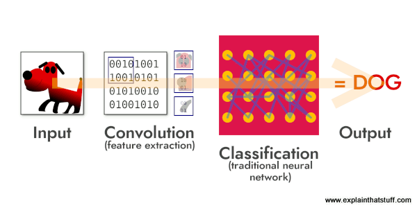
Our CNN can classify CIFAR-10 images with a certain level of accuracy after just a few epochs. In an IoT scenario, similar models could be deployed on small devices like a Raspberry Pi (e.g., using TensorFlow Lite) or used in the cloud for real-time image classification. This example demonstrates how convolutional layers extract features from images, and how pooling layers reduce spatial size while keeping the most important information.

Ideas for IoT Integration:

  • Convert this model to TensorFlow Lite to run on edge devices with limited resources.
  • Use a camera-equipped device (Raspberry Pi or other SBC) to capture real-time images and classify them locally.
  • Send the images or classification results to a remote server for centralized monitoring or logging.

Practice

Below, you have a link to the Jupyter/Colab notebook where you can practice the theory from this section:

CNN classification notebook

Summary

In this section, we've covered the basics of Convolutional Neural Networks, including convolutional and pooling layers. We also explored practical examples of building and training CNNs for image classification. These concepts and techniques are fundamental to understanding and working with CNNs in various computer vision applications.

Feito con eXeLearning (Nova xanela)