Basic Concepts of Neural Networks

Welcome to the second section of our Deep Learning module, where we delve into Artificial Neural Networks, commonly known as ANNs. ANNs are the backbone of Deep Learning, inspired by the biological neural networks that constitute animal brains. At a high level, an ANN is composed of interconnected units called neurons, which are organized in layers.

Each neuron receives input, processes it, and passes on the output to the next layer of neurons. This process allows the network to learn and make predictions. The power of ANNs lies in their ability to learn complex patterns and representations from data, making them suitable for a wide range of applications.

Input, Hidden, and Output Layers

The architecture of an ANN consists of three main types of layers: the input layer, hidden layers, and the output layer. The input layer receives the initial data, which could be anything from an image's pixel values to numerical data points. This data is then passed through one or more hidden layers where the actual computation and learning occur.

Hidden layers are made up of neurons that apply transformations to the input data using weights, biases, and activation functions. These layers allow the network to learn intricate patterns by adjusting the weights during the training process. Finally, the output layer produces the final prediction or classification, depending on the task at hand.

Let’s visualize a simple neural network architecture:

Activation Functions

Activation functions are essential components of neural networks because they introduce non-linearity into the model. This non-linearity allows neural networks to learn complex relationships and patterns in data that cannot be captured by linear models alone. Without activation functions, no matter how many layers a network has, it would behave like a single-layer linear model, which severely limits its capabilities.

Below are the most commonly used activation functions in artificial neural networks, along with their properties:

• Sigmoid Function: Outputs values between 0 and 1, often used in binary classification problems.
• Tanh Function: Outputs values between -1 and 1, providing stronger gradients than the sigmoid function.
• ReLU (Rectified Linear Unit): Outputs zero for negative inputs and the input itself for positive inputs, helping mitigate the vanishing gradient problem.

The choice of activation function depends on the specific layer and task in the network:

• Hidden Layers:
  • ReLU is the default choice for most applications due to its efficiency and ability to avoid vanishing gradients.
  • Tanh can be used if zero-centered outputs are desired.
• Output Layers:
  • Sigmoid is suitable for binary classification.
  • Softmax (not covered here) is ideal for multi-class classification.

Impact on Performance: Activation functions significantly influence:

• Model convergence speed: Some functions (like ReLU) enable faster training.
• Accuracy: A well-chosen function helps the network generalize better to unseen data.

By understanding the strengths and weaknesses of each function, you can make informed decisions when designing neural networks.

Let’s plot these activation functions to understand their behavior:

import numpy as np
import matplotlib.pyplot as plt

x = np.linspace(-10, 10, 100)

# Sigmoid function
sigmoid = 1 / (1 + np.exp(-x))

# Tanh function
tanh = np.tanh(x)

# ReLU function
relu = np.maximum(0, x)

# Plotting
plt.figure(figsize=(10, 6))
plt.plot(x, sigmoid, label='Sigmoid')
plt.plot(x, tanh, label='Tanh')
plt.plot(x, relu, label='ReLU')
plt.title('Activation Functions')
plt.xlabel('Input')
plt.ylabel('Output')
plt.legend()
plt.grid(True)
plt.show()

This code snippet plots the sigmoid, tanh, and ReLU activation functions.

Introduction

In this notebook, we will predict the status of a machine (working or failing) based on temperature and vibration sensor readings. This notebook builds on theoretical concepts from the course, including:

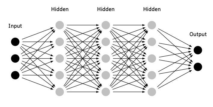
• Neural network architecture
• Activation functions
• Layers and neurons
• Training via backpropagation

We use TensorFlow in this notebook because it simplifies the process of building and training neural networks, making it easier for beginners to focus on core concepts like layers, activation functions, and training. With its high-level Keras API, TensorFlow handles complex operations like backpropagation and gradient updates for us, allowing for readable, intuitive code. This approach helps learners grasp the fundamentals without being overwhelmed by implementation details, while also providing the scalability to explore advanced features later.

Follow along step by step and execute each cell to see the theory in action.

Step 1: Import Libraries

We start by importing the necessary libraries. These include:

• TensorFlow: For building and training the neural network.
• NumPy: For numerical operations and data generation.
• Matplotlib: For data visualization.
• Scikit-learn: For data preprocessing and splitting.

import tensorflow as tf
from tensorflow.keras import Sequential
from tensorflow.keras.layers import Dense, Dropout
import numpy as np
import matplotlib.pyplot as plt
from sklearn.model_selection import train_test_split
from sklearn.preprocessing import StandardScaler
import ipywidgets as widgets
from IPython.display import display, clear_output

print("Libraries imported successfully!")

Step 2: Generate Synthetic Data

We simulate sensor readings for machine status prediction. The data consists of:

• Working Machines: Normal operating ranges (temperature: ~50°C, vibration: ~20 m/s²).
• Failing Machines: Higher temperature and vibration values (temperature: ~75°C, vibration: ~45 m/s²).

This data is generated using random distributions to mimic real-world variability.

def generate_training_data(n_samples=1000):
    np.random.seed(42)
    n_working = int(n_samples * 0.6)
    n_failing = n_samples - n_working

    # Working machines
    temp_working = np.random.normal(50, 5, n_working)
    vib_working = np.random.normal(20, 3, n_working)

    # Failing machines
    temp_failing = np.random.normal(75, 5, n_failing)
    vib_failing = np.random.normal(45, 5, n_failing)

    # Combine data
    X = np.vstack([
        np.column_stack([temp_working, vib_working]),
        np.column_stack([temp_failing, vib_failing])
    ])
    y = np.array([0] * n_working + [1] * n_failing)
    return X, y

X, y = generate_training_data(1000)

# Show data samples
print(f"Temperature samples: {X[:5, 0]}")
print(f"Vibration samples: {X[:5, 1]}")
print(f"Labels: {y[:5]}")

Step 3: Visualize the Data

To understand the data distribution, we plot temperature and vibration readings for both working and failing machines.

plt.figure(figsize=(10, 6))
plt.scatter(X[y==0, 0], X[y==0, 1], c='blue', label='Working Machines')
plt.scatter(X[y==1, 0], X[y==1, 1], c='red', label='Failing Machines')
plt.title("Temperature vs. Vibration")
plt.xlabel("Temperature (°C)")
plt.ylabel("Vibration (m/s²)")
plt.legend()
plt.grid(True)
plt.show()

Step 4: Prepare the Data

Before training, we split the data into:

• Training Set: 80% of the data, used for training the model.
• Testing Set: 20% of the data, used to evaluate the model.

We also normalize the features to ensure all input values are on a similar scale.

X_train, X_test, y_train, y_test = train_test_split(X, y, test_size=0.2, random_state=42)

# Normalize data
scaler = StandardScaler()
X_train_scaled = scaler.fit_transform(X_train)
X_test_scaled = scaler.transform(X_test)

print("Data prepared for training.")

Step 5: Build the Neural Network Model

We build a simple neural network with the following architecture:

• Input Layer: 2 input features (temperature, vibration).
• Hidden Layer: 16 neurons with ReLU activation.
• Output Layer: 1 neuron with Sigmoid activation for binary classification.

model = Sequential([
    Dense(16, activation='relu', input_dim=2),
    Dense(1, activation='sigmoid')
])
model.compile(optimizer='adam', loss='binary_crossentropy', metrics=['accuracy'])
print("Model created.")

Step 6: Train the Model

We train the model using backpropagation for 50 epochs with a batch size of 32. The loss is minimized using binary crossentropy.

history = model.fit(
    X_train_scaled, y_train, 
    epochs=50, 
    batch_size=32, 
    validation_split=0.2,
    verbose=1
)
print("Training complete.")

Step 7: Evaluate the Model

We evaluate the model on the test data to measure its accuracy and ensure it generalizes well.

test_loss, test_accuracy = model.evaluate(X_test_scaled, y_test)
print(f"Test Loss: {test_loss:.4f}, Test Accuracy: {test_accuracy:.4f}")

Step 8: Interactive Prediction

Use the sliders below to input temperature and vibration values. The model will predict whether the machine is working or failing.

def predict_status(temp, vib):
    input_data = np.array([[temp, vib]])
    input_scaled = scaler.transform(input_data)
    prediction = model.predict(input_scaled)[0][0]
    return "Failing" if prediction > 0.5 else "Working"

def create_interface():
    temp_slider = widgets.FloatSlider(value=50, min=30, max=90, step=0.5, description='Temperature (°C):')
    vib_slider = widgets.FloatSlider(value=20, min=10, max=60, step=0.5, description='Vibration (m/s²):')
    output = widgets.Output()

    def update(change):
        with output:
            clear_output()
            status = predict_status(temp_slider.value, vib_slider.value)
            print(f"Temperature: {temp_slider.value}°C")
            print(f"Vibration: {vib_slider.value} m/s²")
            print(f"Prediction: {status}")

    temp_slider.observe(update, names='value')
    vib_slider.observe(update, names='value')
    display(widgets.VBox([temp_slider, vib_slider, output]))

create_interface()

In this section, we covered the basic concepts of neural networks, the architecture of ANNs including input, hidden, and output layers, and the importance of activation functions. We also explored the training process involving backpropagation and gradient descent optimization, supported by practical examples and code snippets. These foundational concepts are essential for understanding how ANNs learn and make predictions.